Hyperelastic material
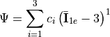
Yeoh strain energy density function:
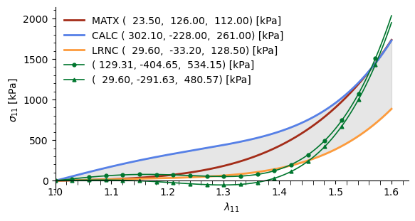
Example of used material parameters and possibile instable combinations created interpolating the coefficient (see myLoading.m):
Hyperelasticity background
Warning
The following is partially taken from my Master thesis.
We consider a continuous body in the reference configuration  that could move in space toward the spatial configuration
 . The map between reference position
 and the spatial position
 of the material particle is represented by the motion
 .
In finite deformations, no assumptions are made on the magnitude of displacement
 , that as no small displacements are required.
At the time  the motion in the neighborhood of a material point is represented by the deformation gradient:

It is the primary measure of deformation and allows to relate the relative position of neighboring particles after and before the deformation in terms of their relative material position.
The local motion could be also decomposed into a rigid body motion and deformation using a polar decomposition of the deformation gradient as

 and
 represent unique, positive definite, symmetric tensors called respectively as right (or material) stretch tensor and left (or spatial) stretch tensor. They measure local stretching along mutually orthogonal eigenvectors.
 is an orthogonal tensor called as rotation tensor representing the rigid body rotation.
Strain
At finite deformations, non-linear strain measures are used to correctly represent the differences between the reference and the spatial configuration.
The right Cauchy-Green strain is formulated with respect to the reference configuration and could be expressed as:

An additional deformation tensor is the Green-Lagrange strain tensor, reading:
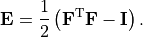
The latter is used to represent the change in the squared lengths  , where
 is the linear stretch and represents how the line element is deformed from the original direction
 to the spatial configuration
 (with
 ). This is:

A line element is extended for  , unstretched for
 or compressed for
 .
The Cauchy-Green strain tensor can be also represented through eigenvalue representation, with the principle stretches  and the principal stretch direction
 , as:

Stress
To represent the load on the material particle a stress measure is required. The Cauchy stress  is a second-order tensor used to represent the stress state containing both the normal stress and the shear stress components acting respectively perpendicular or in parallel to the local area
 as shown in cref{fig:cauchy_stress}.
However, at finite deformation, where the current configuration is different from the reference one, other stress tensors may be defined. While the Cauchy stress is represented in the current configuration, the first Piola-Kirchoff relates the force in the spatial configuration to the area element in the reference configuration. Through the backward Piola transform it could be related to the Cauchy stress as:
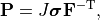
where  and
 is the deformation gradient.
The second Piola-Kirchhoff stress pull-back the force in the spatial configuration to the reference one and so it is entirely expressed in the reference configuration . It could be expressed as:

Furthermore, the Cauchy stress can be represented in a coordinate system within which the shear stress disappears. This stress state is called the principal stress state and the principal stress directions  represent the eigenvectors of the stress state. Introducing the principal stresses
 , the Cauchy stress in a principal coordinate system reads:

Vascular vessels are cylinder-like structures that can be approximated as a typical engineering problem named as pressurized tube. Inflated vessels may be characterized by a mutual tri-orthogonal axial system representing cylindrical coordinates. For this simplified setup, the three principal directions are circumferential, axial and radial one with the related stresses shown in cref{fig:cylindricalStress}. Due to the boundary conditions of the problem the radial stress has to balance the internal pressure inside and the external one outside while the circumferential stresses are generated to resist the resulting bursting effect. Since the internal pressure is higher than the external one, radial stresses are generally higher inside and gradually decrease across the thickness. Circumferential stresses follow a similar trend depending on the internal pressure but also on wall thickness. For a thick-wall cylinder, they could be calculated using the Lam'e equations with the resulting trend in cref{fig:cylindricalStress}.
Governing laws
The motion of a material particle of density  is governed by the linear momentum balance equation:
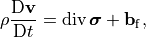
where  is the Cauchy stress tensor, is the particle velocity and
 is the body force per unit volume.
The balance of angular momentum is a priori satisfied by the symmetry of the Cauchy stress tensor:  .
Boundary Value Problem
In continuum mechanics, the primary unknown variable is the displacement field  and this can be obtained from the solution of the Boundary Value Problem (BVP) derived from the balance of linear momentum and constitutive relations.
The body is characterized by the boundary  , split into
 and
 . At Dirichlet or essential boundary conditions are prescribed in order to impose the displacement, while at Neumann or natural boundary conditions prescribe the traction through the boundary normal.
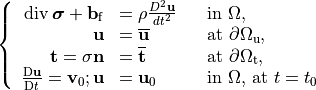
For a transient problem, the mathematical description should be closed by the initial conditions on the velocity and displacement field. hence, the BVP is described by the following set of equations:
Finite Element Method
The Finite Element Method is a widely used method to numerically solve partial differential equations (PDE). It is a procedure based on the representation of the continuum with a finite number of points, called nodes, within the continuum body in order to discretize the full body (of arbitrary geometry) by means of a finite set of sub-regions of standard geometries called finite elements. Over every region, both the geometry and the variables of the governing equations are approximated in order to solve complex systems of equations over elaborate domains.
The governing equations are usually reformulated in the weak integral form and the finite element approximation leads to a finite set of non-linear algebraic equations in the primary variable. Then, these equations could be solved with an iterative technique such as the Netwton-Rapson method.
Spatial description
The domain is approximated as a discretized domain segmented into  subdomains:
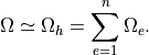
This discretization allows us to focus only on a single finite element  for the governing equations and material description.
The primary variables are approximated through the shape functions  . The latter interpolate the primary variables in space over the finite element through their values at nodes as:
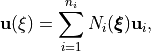
where  represents the coordinates in the single element domain with in
 nodes.
By storing all the independent variables  into a vector
 of dimension
 the finite element interpolation can be reformulated as

with the interpolation matrix  collecting shape functions .
By using an isoparametric finite element formulation, both the essential variables and the spatial coordinates use the same shape function, so:
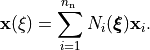
The shape functions could be defined in the natural coordinate of the finite element  and linked to the global coordinate through the Jacobian
 . It allows us to define shape function and further numerical quadrature only for each specific typology of finite element, and then map it to the current geometries.
Due to the interpolation in cref{eq:interpolation} also the symmetric spatial gradient of the essential variables could be expressed through an interpolation matrix as:

where expresses the  independent components of the gradients as a single vector with the convention of
 .
 represents the gradient interpolation matrix and stores the gradient of the shape functions. This gradient requires the Jacobian matrix because the shape functions are expressed with respect to the natural coordinates but they are derived with respect to the global coordinate . Each row of is expressed as:

Calculus of variations
Physical problems are often described by local governing equations with the description in the so-called strong form of the problem. However, FEM requires the weak or integral form in order to discretize and then solve the problem. A general method to derive the weak form is the Calculus of Variations. Multiplying the governing equations with a test function, and then integrating over the body domain, leads to the weak form of the problem.
For a solid mechanics problem, the body occupies the initial configuration and the problem is formulated with respect to the essential variable, the displacement . The state of motion is described by the displacement and its time derivatives, velocity  and acceleration
 .
They have to satisfy the equilibrium equation.
Furthermore, a Dirichlet boundary
 allows for prescribed displacement condition
 and a Neumann boundary
 for traction condition oriented across the outward-normal
 .
This leads to the BVP as expressed in cref{eq:BVP}.
The equilibrium equation is then multiplied with an admissible variation  and it is integrated over the body domain.

The first term can be split following the integration by parts:

Furthermore, the divergence theorem can be applied:

Then, the weak form can be expressed as:

where the two  terms represent respectively the external and internal work upon the admissible variation.
It is also interesting to observe that cref{eq:weakform} correspond to the principle of virtual work when the admissible variation is regarded as corresponding to an admissible variation of the engineering strain  .
The weak form is irreducible and involves only the first-order derivative of the essential variable. So, the derivative order of the displacement field appears to be reduced with respect to the strong from and shared with the derivative of the test function.
In non-linear mechanical problems, where large deformations are involved together with non-linear constitutive models, it is convenient to express the internal work term with respect to the reference configuration through the second Piola-Kirchhoff stress and the variation of the Green-Lagrange strain, as:

where  is the admissible variation of the Green-Lagrange strain.
The balance equation obtained from Eq. eqref{eq:deltaPi} is nonlinear and, to be solved, has to be linearized along the increment of the displacement, that is:

With the direction derivative  along the increment of displacement
 :

where  is the non-linear material stiffness.
By pushing it forward to the spatial configuration:

There are two different contributions to the linearized internal work, that is a geometric contribution:

and a material contribution:

Both terms depend on the choice of the constitutive model to be determined.
Discretization
Galerkin’s approach uses the same interpolation for essential variable and their test function. In other words, the nodal displacements, stored in , and their admissible variations, stored in  , are interpolated with the same interpolation functions, collected in .
Then the discretized weak form for the
 finite element reads:

The  term contains two different contributions. The material contribution leads to the material stiffness matrix of the finite element:
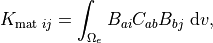
where  denotes the material stiffness linked to the constitutive model.
The geometrical contribution denotes the geometric stiffness matrix:

where  are the component of the Cauchy stress.
These integrals are commonly computed through numerical quadrature formulas.
Given  arbitrary admissible variation , the discretized weak form yields to a system of algebraic equations:

This system of equations can be solved with numerical iterative methods. If the velocity and acceleration terms are different from zero also a time discretization is required. \
A non-linear stationary FEM problem can be expressed as:

and iteratively solved through a numerical procedures that minimize the residuum  , ideally until
 . Adopting a Newton-Rapson iterative scheme, the current solution at step
 is computed from the previous step
 as:

with the increment  :

Both the material and the geometrical stiffness matrixes are functions of the essential variable and need to be evaluated in each step of the iterative solver. Furthermore, also a load increment approach could be used. The external boundary load is incremented with a load factor and an equivalent system is solved for each load step, as two nested loops. newline
Further technical details for implementation with the Comsol finite element solver are described in the appendix.
Kinematic decomposition
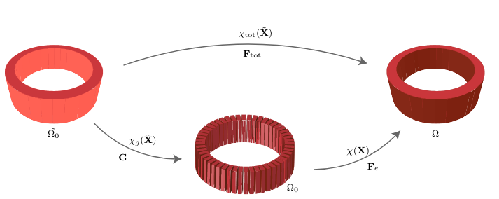
Representation of the tissue growth and remodeling through a kinematic description. The stress-free intermediate (eventually incompatible) configuration Ω0 separates the growth-related and the non-growth-related motions. The deformation gradient is multiplicatively decomposed and the final deformation is due to both the deformation gradient and the growth tensor.
The total deformation gradient reads:

where  is the elastic deformation gradient and
 is the growth tensor.
The elastic deformation gradient can be exprssed as:
