AceGEN Elements

An example of the element code is shown here.

O2P1YG

The O2P1YG element is a solid wall element with 3D quadratic tetrahedra used to describe the atherosclerotic wall, including heterogeouns material and a G&R algorithm.

Main characteristics:

3D quadratic tetrahedrons with 10 nodes
Quadratic shape functions for displacements
Linear shape functions for auxiliary pressure (incompressibility constraint)
Finite strain formulation
Hyperelastic material model based on the Yeoh strain energy density function
Element-based material properties assignment
Growth & remodelling capabilities based on the multiplicative decomposition of the deformation gradient and the homogenous stress hypothesis.
Local (Gauss point) solution for the growth tensor

Discretization

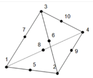
The element requires an O2-type of mesh, with the sequence indicated in:

Warning

The element requires "SMSNoElementData" -> 8 assigned in the SMSTemplate.

The ElementData[[i]] elements are used to:

1 to 3 to represent the material coefficients $c_1$ , $c_2$ , and $c_3$ in the Yeoh strain energy density function
4 to activate/deactivate the growth algorithm ( $\alpha$ parameter)
5 to read the average first principal stress (from the post-processing routines)
6 to read the first principal stress in the element (from the post-processing routines)
7 to read the lower threeshold to map the growth magnitude
8 to read the upper threeshold to map the growth magnitude

Note

The usage of the SMSIO["ElementData"][[6]] to read the average first principal stress in the element can be replace by an internal reading of the stress. This is still in development. However, using the external reading (within the post-processing routines) make the element more stable.

Kinematics

{ξ, η, ζ} ⊨ SMSIO["Integration point"[Ig]];
wgp ⊨ SMSIO["Integration weight"[Ig]];
{𝕏IO, 𝕡eIO} ⊨ SMSIO["All coordinates and DOFs"];
𝕡e = Flatten[𝕡eIO];

(*SHAPE FUNCTIONS*)
k ⊢ 1 - ξ - η - ζ; ℕh ⊨ { (2 ξ - 1) ξ, (2 η - 1) η, (2 ζ - 1) ζ, (2 k - 1) k, 4 ξ η,  4 η ζ, 4 ζ ξ, 4 ξ k, 4 η k, 4 ζ k};
Np ⊨ {1 - ξ - η - ζ, ξ, η, ζ};

(*ISOPARAMETRIC MAPPING*)
𝕏IOgeo ⊨ 𝕏IO[[1 ;; nenX, 1 ;; ndim]];
𝕏 ⊨ SMSFreeze[ℕh . 𝕏IOgeo];
𝕁e ⊨ SMSD[𝕏, {ξ, η, ζ}];  Jed \
⊨ SMSDet[𝕁e];

(*KINEMATICS*)
𝕦IO ⊨ 𝕡eIO[[1 ;; nenU, 1 ;; ndim]];
𝕦 ⊨ ℕh . 𝕦IO;
ℍ ⊨ SMSD[𝕦, 𝕏, "Dependency" -> {{ξ, η, ζ}, 𝕏, SMSInverse[𝕁e]}];
𝔽 ⊨ SMSFreeze[IdentityMatrix[3] + ℍ];
𝕁F ⊨ SMSDet[𝔽]; ε = SMSVariables[𝔽];

(*MIXED VARIABLE*)
pIO ⊨ 𝕡eIO[[nenU + 1 ;; nen, 1]]; p ⊨ Np . pIO;

ℂ ⊨ Transpose[𝔽] . 𝔽; 𝔽ISO ⊢ 𝕁F^(-1/3) 𝔽;
SMSFreeze[ℂISO, Transpose[𝔽ISO] . 𝔽ISO, "Symmetric" -> True];

Warning

It’s important to specifiy the dependencies using of $\mathbb{H}=\nabla \mathbf{u}$ . It’s important to use SMSFreeze to set variables like $\mathbb{F}$ and $\mathbb{C}$ , we’ll use them to calculate symbolic derivatives

Note

The variable ${\epsilon}$ containts a list with the deformation gradient components $\mathbb F_{11}, \mathbb F_{22}, \mathbb F_{33}, \mathbb F_{12}, \mathbb F_{23}, \mathbb F_{13}$ . These variables are used in the growth variables compuation.

Constitutive equations

The constitutive equations are based on the Yeoh strain energy density function:

$\Psi = {c_1} (\bar{I}_{1e} - 3) + {c_2}(\bar{I}_{1e} - 3)^2 + {c_3}(\bar{I}_{1e} - 3)^3 + p (\mathbf{JF}_e - 1)$

where $\bar{I}_{1e} = \text{tr}(\bar{\mathbb{C}}_e)$ is the first isochoric invariant of the elastic right Cauchy-Green tensor, $\mathbf{JF}_e$ is the determinant of the elastic deformation gradient and $p$ is the auxiliary pressure.

This functions is implemented in the Growth[task_, hg_] function as:

𝕀 ⊨ IdentityMatrix[3];
α ⊨ SMSIO["Element data"][[4]];
𝔽in ⊨ 𝕀 + {{𝕙g[[1]], 𝕙g[[2]], 𝕙g[[3]]}, {𝕙g[[4]], 𝕙g[[5]], 𝕙g[[6]]}, {𝕙g[[7]], 𝕙g[[8]], 𝕙g[[9]]}};
𝔽e ⊨ 𝔽 . SMSInverse[𝔽in];
𝕁Fe ⊨ SMSDet[𝔽e];
𝔽ISOe ⊨ 𝕁Fe^(-1/3) 𝔽e;
SMSFreeze[ℂISOe, Transpose[𝔽ISOe] . 𝔽ISOe,"Symmetric" -> True];
𝕀ISOe ⊨ Tr[ℂISOe];
Ψe ⊨ c1 (𝕀ISOe - 3) + c2 (𝕀ISOe - 3)^2 + c3 (𝕀ISOe - 3)^3 + p (𝕁Fe - 1);

where the growth variables are computed used an internal Gauss point solution for the growth tensor $\mathbb{F}\mathrm{in}$ .

Growth & Remodelling

The function Growth[task_, hg_] setting task="Q" return the growth tensor equations with its incremental formulation (see here).

The growth magnitude is computed as:

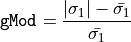
$\texttt{gMod} = \frac{|\sigma_1|-\bar{\sigma_1}}{\bar{\sigma_1}}$

where $\bar{\sigma_1}$ is the stress averaged across all the MATX elements and $\sigma_1$ is the first principal stress in the element.

This is mapped using a distribution map with the lower and upper threeshold:

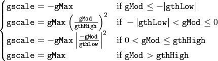
$\begin{cases} \texttt{gscale} = -\texttt{gMax} & \text{if } \texttt{gMod} \leq -|\texttt{gthLow}| \\ \texttt{gscale} = \texttt{gMax}\left(\frac{\texttt{gMod}}{\texttt{gthHigh}}\right)^2 & \text{if } -|\texttt{gthLow}|< \texttt{gMod} \leq 0 \\ \texttt{gscale} = -\texttt{gMax}\left|\frac{-\texttt{gMod}}{\texttt{gthLow}}\right|^2 & \text{if } 0< \texttt{gMod} \leq \texttt{gthHigh} \\ \texttt{gscale} = \texttt{gMax} & \text{if } \texttt{gMod} >\texttt{gthHigh} \end{cases}$

where:

gthLow ⊨ SMSIO["Element data"][[7]];
gthHigh ⊨ SMSIO["Element data"][[8]];
gMax ⊢ 0.01;
gMod ⊢ ((SMSAbs[σ1] - σ1AV)/σ1AV);

Note

The gMax variable is set to $0.01$ to avoid large growth values. This value can be adjusted according to the problem. This values was introduced only toincrease the stability.

The the growth tensor is then assebled to described the local Gauss point equations in its incremental form:

$\mathbf{F}{g}_{(n+1)} = \mathbf{F}e^{-1}_{(n+1)} \exp[ \mathbf{l}{g}_{(n+1)} \Delta t ] \mathbf{F}{e}_{(n+1)} \mathbf{F}{g}_{n}$

in the element code, the growth tensor is computed as:

𝕝g ⊨ α gscale 1/(SMSAbs[σMain[[1]]] + SMSAbs[σMain[[2]]] + SMSAbs[σMain[[3]]]) Sum[SMSAbs[σMain[[k]]] Table[σMainDir[[k, i]] σMainDir[[k, j]], {i, 1, 3}, {j, 1, 3}], {k, 1, 3}];
If[task == "f", Return[SMSDet[𝕝g]]];
𝔽inN ⊨ 𝕀+ {{𝕙gnIO[[1]], 𝕙gnIO[[2]], 𝕙gnIO[[3]]}, {𝕙gnIO[[4]], 𝕙gnIO[[5]], 𝕙gnIO[[6]]}, {𝕙gnIO[[7]], 𝕙gnIO[[8]], 𝕙gnIO[[9]]}}; (* from old step *)
𝔽g ⊨ SMSInverse[𝔽e] . SMSMatrixExp[𝕝g Δt,1] . 𝔽e . 𝔽inN;
ℚ ⊨ 𝔽in - 𝔽g;
If[task == "Q", Return[Flatten[ℚ]]];

Warning

The computation of $\exp[\mathbf l_g\Delta t]$ is the exponetial of a tensor. This may be (is) really compuationally expensive. Using SMSMatrixExp is a good way to avoid numerical issues.

Note

Returing $\mathbf Q = \mathbf F_{in} - \mathbf F_g$ allows to compute the equations by enforcing $\mathbf Q = 0 \rightarrow \mathbf F_{in} = \mathbf F_g$ in the local Newton-Raphson scheme described in the following.

To solve for the growth tensor variables, the element uses a local Newton-Raphson scheme to solve the equations:

$\mathbf{Q} = 0$

using an iterative schema:

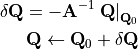
$\delta \mathbf Q = - \mathbf A^{-1} \left.\mathbf Q\right|_{\mathbf Q_0}\\ \mathbf Q \leftarrow \mathbf Q_0 + \delta \mathbf Q$

where $\mathbf A$ is the Jacobian matrix of the $\mathbf Q$ .

This is implement in the element code inside the GaussPointComputation[ig_] function as:

SMSIf[α == 0 || (iNR == 1 && staten == 0)(*||(iNR>1 && ftr<tol)*)];
    (*Elastic step*)
    𝕙g ⫤ 𝕙gnIO; SMSIO[Join[𝕙g, {0}], "Export to", "Element time dependent data"[Table[Ihg + i, {i, lhg}]]];
SMSElse[];
(*Growth step*)
    𝕙gb ⫤ 𝕙gnIO;
    SMSDo[jNR, 1, 30, 1, 𝕙gb];
        ℚg ⊨ Growth["Q", 𝕙gb];
        𝔸g ⊨ SMSD[ℚg, 𝕙gb];
        Δ𝕙 ⊨ SMSLinearSolve[𝔸g, -ℚg];
        𝕙gb \[LeftTee] 𝕙gb + Δ𝕙;
        SMSIf[SMSSqrt[Δ𝕙 . Δ𝕙] < tol];
            SMSIO[Join[𝕙gb, {1}], "Export to","Element time dependent data"[Table[Ihg + i, {i, lhg}]]];
            D𝕙Dε ⫤ SMSLinearSolve[𝔸g, -SMSD[ℚg, ε, "Constant" -> 𝕙gb(*,"Method"->"Forward"*)]];
            SMSBreak[];
        SMSEndIf[D𝕙Dε];
        SMSIf[jNR == "29"];
            SMSExport[{1, 2}, {idata$$["SubDivergence"], idata$$["ErrorStatus"]}];
            SMSBreak[];
        SMSEndIf[];
    SMSEndDo[𝕙gb, D𝕙Dε];𝕙g \[LeftTee] SMSFreeze[𝕙gb, "Dependency" -> {ε, D𝕙Dε}];
SMSEndIf[𝕙g];

Caution

Once the computation is done, $\mathbf{h}_g$ needs to be freezed (SMSFreeze) using the dependencies of the growth tensor variables expressed in $\mathbb{D}{h}\mathbb{D}\epsilon$ .

Tangent and residual

The tanged and residual computation pre-define the element equations using ElementDefinitions[Ig]; that includes all the kinematics, constitutive equations, and growth variables, the computed the residual and tangent matrix as:

SMSDo[
    Rgi ⊨ Jed wgp SMSD[Ψe, 𝕡e, i, "Constant" -> 𝕙g(*,"Method"->"Forward"*)];
    SMSIO[Rgi, "Add to", "Residual"[i]];
        SMSDo[
            Kgij ⊨
            SMSD[Rgi, 𝕡e, j(*,"Method"->"Forward"*)];
            SMSIO[Kgij, "Add to", "Tangent"[i, j]];
        , {j, i, ndof}];
, {i, 1, ndof}]; SMSEndDo[];

Warning

To ensure the correctness of the symbolic derivatives for the tangent matrix, it is important to set "Constant" -> hg in the SMSD function.

Output

Several post-processing quantities are computed. See the full example here.

Tasks

In order to export the first principal stress for each element a SMSMTaks is implemented as:

(** ... TASKS ... **)
SMSIf[task == 1];
    σpb ⊢ 2 𝕁F^-1 𝔽 . SMSD[Ψe, ℂISOe, "Symmetric" -> True, "Constant" -> 𝕙g] . Transpose[𝔽];
    σ ⊢ (σpb - Tr[σpb] 𝕀/3) + p 𝕀;
    σMain ⊢ SMSEigenvalues[σ];
    SMSIO[Jed wgp σMain[[1]], "Add to", "Task real output"[1]];
SMSEndIf[];

BoundaryPressureP2

A 3D quadratic triangle is used to apply the boundary pressure in the lumen side.

Discretization

The representation of the nodal position with the shape functions allows for its symbolic derivating leading to the computation of the normal directions.

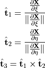
$\hat{\mathbf{t}}_1 = \frac{\frac{\partial \mathbf{X}}{\partial \xi}}{{\|\frac{\partial \mathbf{X}}{\partial \xi}\|}} \\ \hat{\mathbf{t}}_2 = \frac{\frac{\partial \mathbf{X}}{\partial \eta}}{{\|\frac{\partial \mathbf{X}}{\partial \eta}\|}} \\ \hat{\mathbf{t}}_3 = \hat{\mathbf{t}}_1 \times \hat{\mathbf{t}}_2$

And this allows to direct the pressure, readed as DomainData along the third (out-of-plane) direction:

$\mathbf{p} = \left[\begin{array}{ccc} \hat{\mathbf{t}}_1 & \hat{\mathbf{t}}_2 & \hat{\mathbf{t}}_3 \end{array} \right]^T \left[\begin{array}{ccc} 0 & 0 & \mathrm{press} \end{array} \right]$

Implemented as:

𝕩 ⊢ SMSFreeze[𝕏];
{Rξ, Rη} ⊨ Transpose[SMSD[𝕩, {ξ, η}]];
Rζ ⊨ Rξ\[Cross]Rη;
Rn ⊨ Rζ\[Cross]Rξ;
{t1, t2, t3} ⊨ {Rξ/SMSSqrt[Rξ . Rξ], Rn/SMSSqrt[Rn . Rn], Rζ/SMSSqrt[Rζ . Rζ]};
Q ⊨ {t1, t2, t3};
𝕛 ⊨ SMSSqrt[Rζ . Rζ];
p ⊨ Transpose[Q] . {0, 0, -press};

Then the energy is defined as:

$\Phi = -\mathbf{p}\cdot \mathbb{u}$

Allowing to automatically integrate the pressure over the elment area withint the residual computation:

SMSDo[
    Rgi ⊨ 𝕛 wgp SMSD[Ψe, pe, i, "Constant" -> Flatten[{p}]];
    SMSIO[Rgi, "Add to", "Residual"[i]];
    SMSDo[
    Kgij ⊨ SMSD[Rgi, pe, j];
    SMSIO[ Kgij, "Add to", "Tangent"[i, j]];
    , {j, i, ndof}];
, {i, 1, ndof}];    SMSEndDo[];

Caution

The pressure vector is passed as a constant variable in the SMSD function to ensure the correct computation of the symbolic derivatives.

Load follower

To define the load follower pressure boundary element it is necessary to redefine the position as the updated one:

𝕩 ⊢ SMSFreeze[𝕏 + u]; (* current position *)

Warning

This may lead to instability of the solution.

Note

Further test are needed to ensure how and if it can be applied to the current element.

Element example

See the full example here.